POST: https://www.linkedin.com/posts/tom-yeh_deeplearning-generatieveai-llms-activity-7141461533112381441-J35v

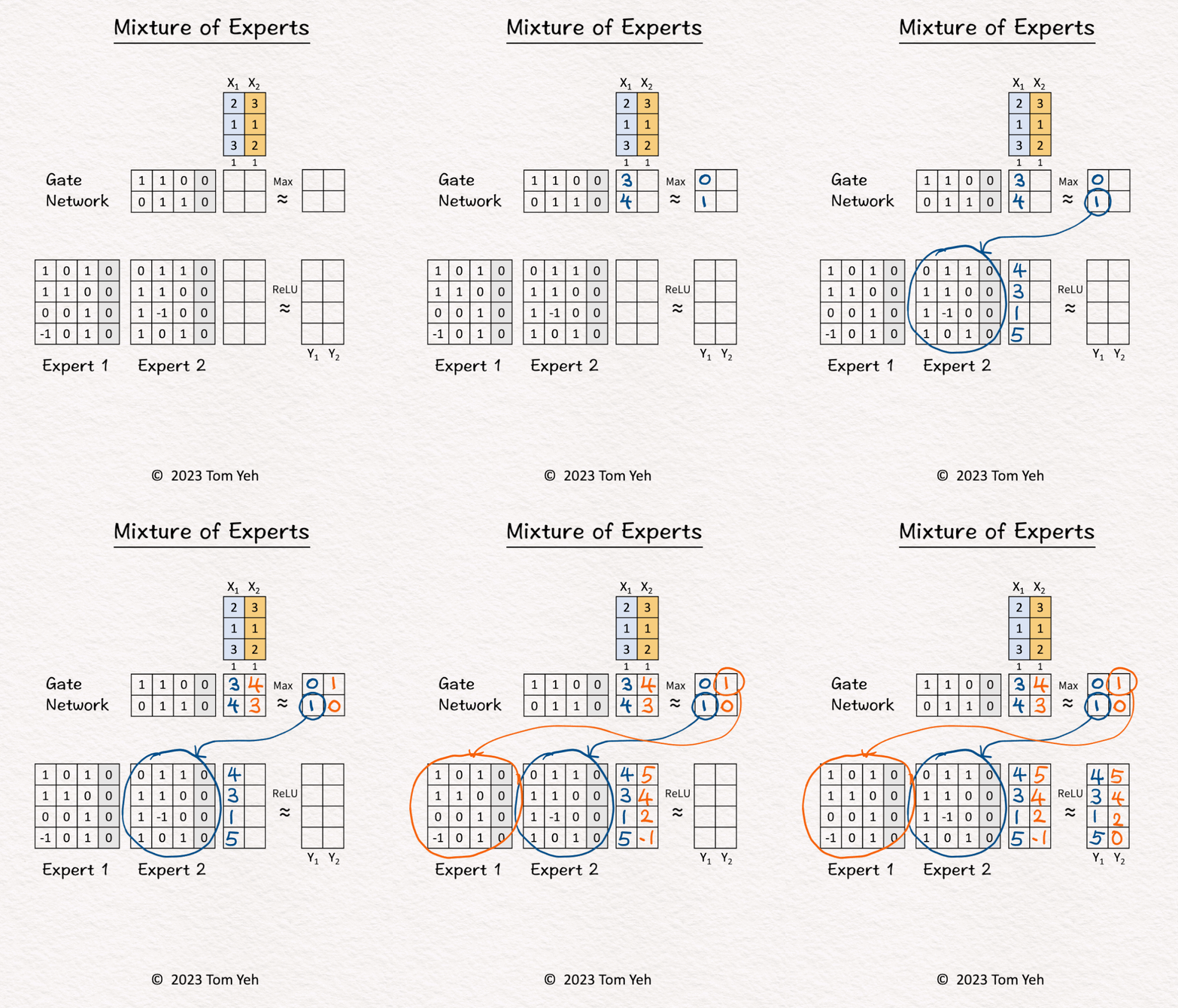
Can you calculate an MoE model by hand? ✍️
[Expert x2, Token x2, Sparse]

Today is our university’s “Reading Day, no class, no assignment due. Students in my Computer Vision and Generative AI courses are all supposed to be studying for the final exams.

Lately I am getting questions about MoE models from my students and LinkedIn followers (David G.)

Why are people interested in MoE Models?

On 12/11, Mistral AI released 8 times bigger 8x7B MoE model. It closed a $415 million series-A. Several people reported this (Sophia Yang, Ph.D., Lewis Tunstall, Marko Vidrih).

How does an MoE model work?

Here is my hands-on exercise to teach my students the basis of MoE models.

𝗦𝘁𝗲𝗽-𝗯𝘆-𝗦𝘁𝗲𝗽 𝗪𝗮𝗹𝗸𝘁𝗵𝗿𝗼𝘂𝗴𝗵

1. [Inputs] The MoE block received two tokens (blue, orange).
2. Gate Network processed X1 (blue) and determined Expert 2 should be activated.
3. Expert 2 processed X1 (blue).
4. Gate Network processed X2 (orange) and determined Expert 1 should be activated.
5. Expert 1 processed X2 (orange).
6. ReLU activation function processed the outputs of the experts and produced the final output.

𝗞𝗲𝘆 𝗣𝗿𝗼𝗽𝗲𝗿𝘁𝗶𝗲𝘀

💡 𝗦𝗶𝘇𝗲: The model can get really large simply by adding more experts. In this example, adding one more expert means adding 16 more weight parameters.

💡𝗘𝗳𝗳𝗶𝗰𝗶𝗲𝗻𝗰𝘆: The gate network will select a subset of experts to actually compute, in this simple exercise, one expert. In other words, only 50% of the parameters are involved in processing a token.   

Taking the two properties together, we can see a sparse MoE can become really large without sacrificing efficiency.

I hope you enjoy this hands-on exercise.

What should I share next?
• More advanced MoE exercises?
• Connect this exercise to math?
• Transformer?
• CLIP?
• Mamba?
• Diffusion?
• Or what else?

POST: https://www.linkedin.com/posts/tom-yeh_deeplearning-neuralnetworks-generativeai-activity-7142506286788620288-jLN4

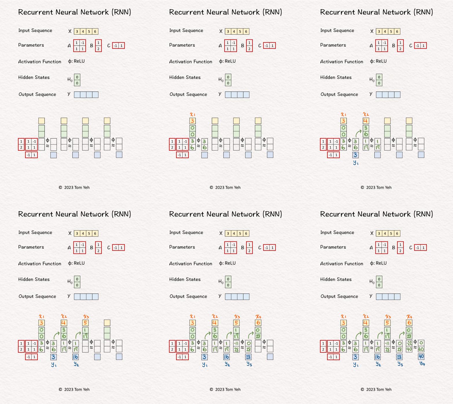
Can you calculate an RNN by hand? ✍️
[Like] if you can follow the calculation

Today is the final exam for the Computer Vision course. I hope my students are ready!

Even though RNN was not originally invented for Computer Vision tasks, I believe it is important for students in my Computer Vision course to practice calculating an RNN by hand to gain a good intuition about how an RNN processes a sequence. Later, when I teach students how to calculate a vision transformer (ViT) model, it is easier for students to see the differences, especially how a transformer processes all tokens in parallel.

Moreover, several people recommended me to do a post about Mamba (Pascal Biese, Steve Solun). RNN is a prerequisite to understand Mamba.

𝗪𝗮𝗹𝗸𝘁𝗵𝗿𝗼𝘂𝗴𝗵

1. Hidden state are initialized to [0, 0].
2. The first input 𝘹1 and hidden states [0, 0] are linearly combined using weights 𝘈 and 𝘉, followed by a non-linear activation function ReLu, to calculate the new hidden states -> [3, 6].
3. Hidden states [3, 6] are linearly combined using weights 𝘊 to obtain the first output 𝘺1
4. Repeat 1-3 for 𝘹2, 𝘹3, 𝘹4

𝗞𝗲𝘆 𝗣𝗿𝗼𝗽𝗲𝗿𝘁𝗶𝗲𝘀

💡Parameters: The same set of parameter matrices (A, B, C) are reused to process each input token. This is the main reason why we use the word 𝘳𝘦𝘤𝘶𝘳𝘳𝘦𝘯𝘵.

💡Sequential: An RNN sequentially processes each input token and produces each output token in turn. An RNN can not process all tokens in parallel. In contrast, the Transformer model can process all tokens in parallel using attention.

Let me know if you have any questions!

Stay tuned for my next post about Mamba!

POST: https://www.linkedin.com/posts/tom-yeh_deeplearning-neuralnetworks-generatieveai-activity-7142854622003560448-PuSc/

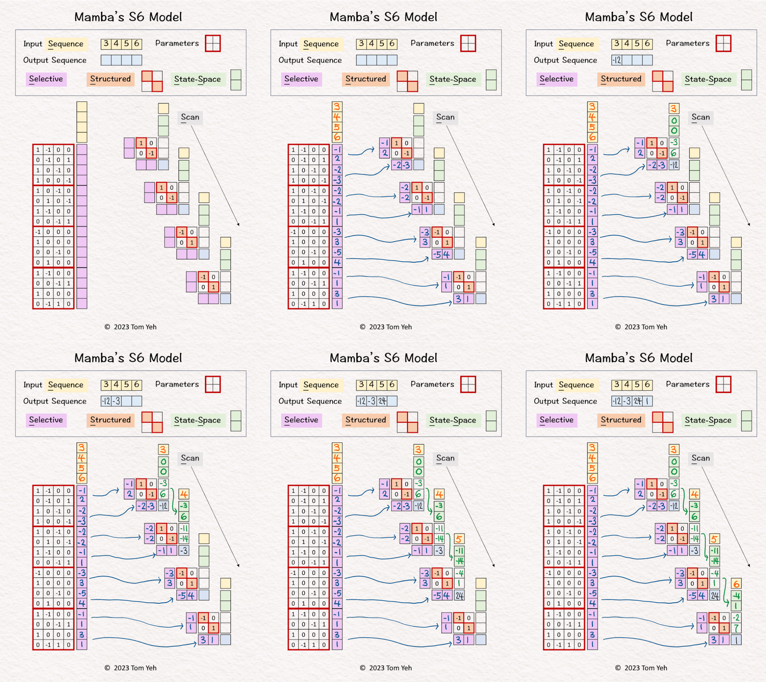
Can you calculate Mamba’s S6 model by hand? ✍️
[1D, 4 tokens, 2 hidden states]

Just one more thing to do before my Computer Vision course ends this semester—grading! But before I get consumed by grading for the rest of the day, let me share my hands-on exercise on Mamba as promised (Pascal Biese, Steve Solun).

The Mamba paper was released on arxiv on Dec. 1. It has since generated quite a buzz, such as posts by Agnieszka Mikołajczyk, Evandro Barros. It is touted as the first linear-time model that beats the transformer model (which is based on a quadratic-time attention mechanism).

At its core, Mamba is based on the new S6 model, which stands for Structured State-Space Sequence modeling using Selective Scan.

I want to thank the first-author of the Mamba paper, Prof. Albert Gu at CMU, for verifying the accuracy of my understanding of how Mamba’s S6 model works. 🙏

— 𝗪𝗮𝗹𝗸𝘁𝗵𝗿𝗼𝘂𝗴𝗵 —

1. Left: All four tokens in the input sequence are processed by a linear layer to calculate a set of weights.
2. Right: These weights are used to drive an RNN-like network.
3. The first input [3] and hidden states [0, 0] are linearly combined using weights A=[-1; 2] and B=[1, 0; 0, -1]  to calculate new hidden states -> [-3, 6]. Note that NO non-linear activation function is involved.
4. Hidden states [-3, 6] are linearly combined using weights C = [-2, -3] to obtain the first output [-12]
5. Repeats steps 3 and 4 using different sets of weights A, B, C.

— 𝗖𝗼𝗺𝗽𝗮𝗿𝗶𝘀𝗼𝗻𝘀 𝘁𝗼 𝗮𝗻 𝗥𝗡𝗡 —

(Pre-requesite: My previous post about RNN)

💡 𝗣𝗮𝗿𝗮𝗺𝗲𝘁𝗲𝗿𝘀: Rather than reusing the same set of weight parameters, each step in the sequence uses a different set of weight parameters. These parameters are “predicted” from the entire input sequence, rather than being trained directly as in the case of a convetional RNN.

💡 𝗟𝗶𝗻𝗲𝗮𝗿𝗶𝘁𝘆: Unlike a conventional RNN, S6 does not use any non-linear activation function.

— 𝗦𝟲’𝘀 𝗦𝗶𝘅 𝗦’𝘀 —

1️⃣ 𝗦𝗲𝗹𝗲𝗰𝘁𝗶𝘃𝗲: Weights in each step are selectively set by a linear layer.

2️⃣ 𝗦𝗰𝗮𝗻: Because each step’s weights are different, it needs to scan through the input sequence to calculate each output token.

3️⃣ 𝗦𝘁𝗿𝘂𝗰𝘁𝘂𝗿𝗲𝗱: The “A” matrices, which are the square matrices used to combine hidden states, assume a certain structure to simplify calculation. In the paper, the assumed structure is diagonal.

4️⃣ 5️⃣ 𝗦𝘁𝗮𝘁𝗲-𝗦𝗽𝗮𝗰𝗲: There are “hidden states” that mutate.

6️⃣ 𝗦𝗲𝗾𝘂𝗲𝗻𝗰𝗲: It is a sequence-to-sequence model.

Note that S6 extends the previous S4 model. The first two S’s–Selective, Scan, are new.

Thanks for reading! Feel free to leave your questions in the comments!

Reference:
[1] Albert Gu, Tri Dao, Mamba: Linear-Time Sequence Modeling with Selective State Spaces. arXiv:2312.00752

POST: https://www.linkedin.com/posts/tom-yeh_deeplearning-generatieveai-llms-activity-7149135567824334848-Wx2B

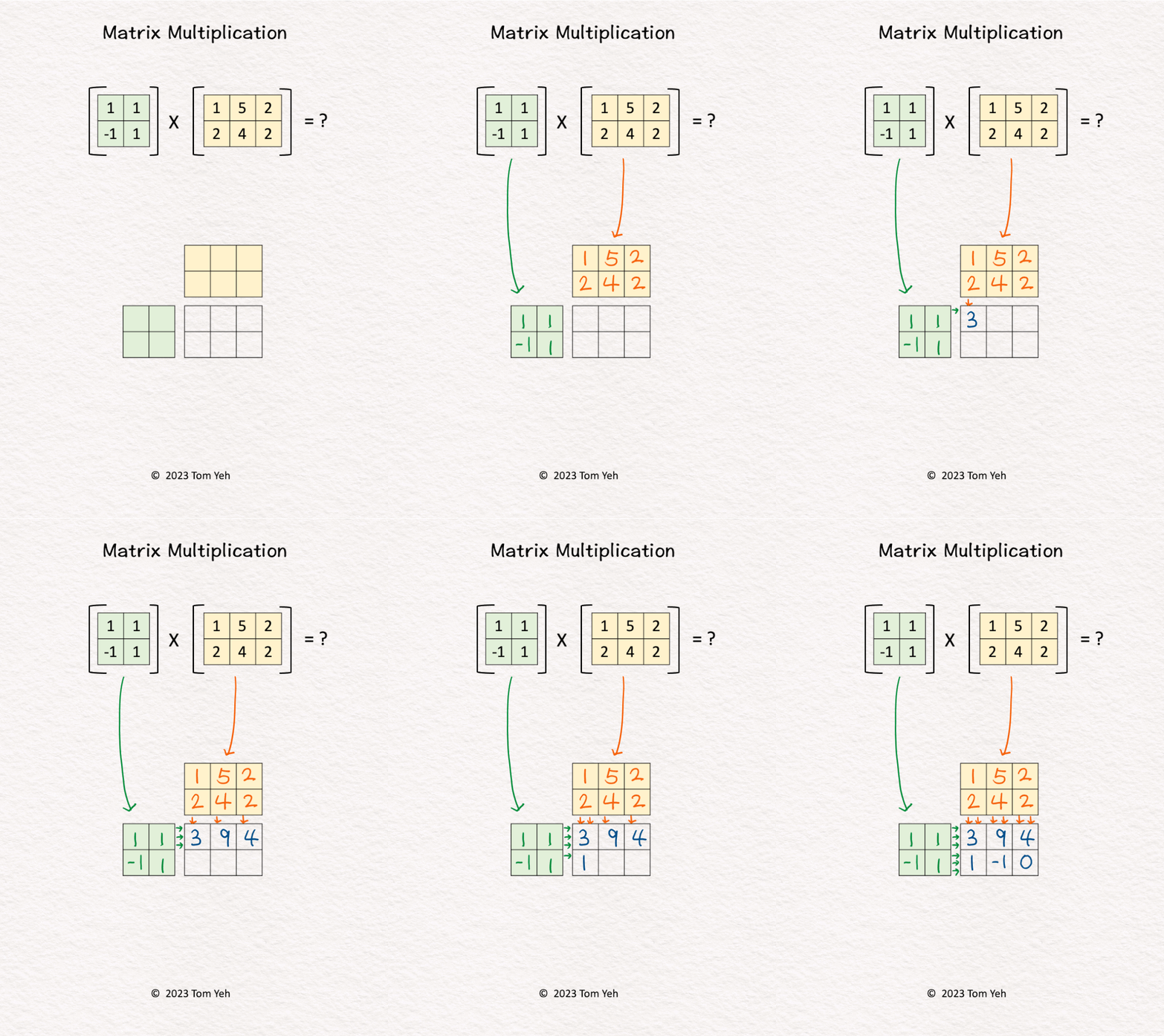
 Can you multiply these matrices by hand? ✍️
[Like] this post if you can calculate this.

One of the key ingredients of the deep learning revolution is the ability to perform matrix multiplications at incredible speed and scale.

Despite linear algebra listed as a prerequisite of my courses, I found many students lack confidence in multiplying matrices. Thus, I teach my students this unique system to multiply matrices by hand.

Let’s say we are calculating A x B = C. This system offers several desirable properties:

💡 𝗗𝗶𝗺𝗲𝗻𝘀𝗶𝗼𝗻𝘀: We can easily see C’s dimensions must match A’s height (vertical) and B’s width (horizontal).

💡 𝗦𝗰𝗮𝗹𝗮𝗯𝗹𝗲: If we scale any of the matrices A, B, C to an arbitrary size, we can easily see how the sizes of other matrices must change accordingly to match the dimensions.

💡 𝗥𝗼𝘄 𝘃𝘀. 𝗖𝗼𝗹𝘂𝗺𝗻 𝗩𝗲𝗰𝘁𝗼𝗿𝘀: For each value in C, we can easily see the corresponding row vector (green) and column vector (yellow) that are combined using dot-product to obtain the value.

💡 𝗦𝘁𝗮𝗰𝗸𝗮𝗯𝗹𝗲: Because of their compactness, we can stack multiple grids like these to represent the underlying sequence of matrix multiplications of a deep neural network (e.g., multi-layer perceptron), like the one I shared a while ago.

POST: https://www.linkedin.com/posts/tom-yeh_deeplearning-generativeai-llms-activity-7149521168889188352-4vc9

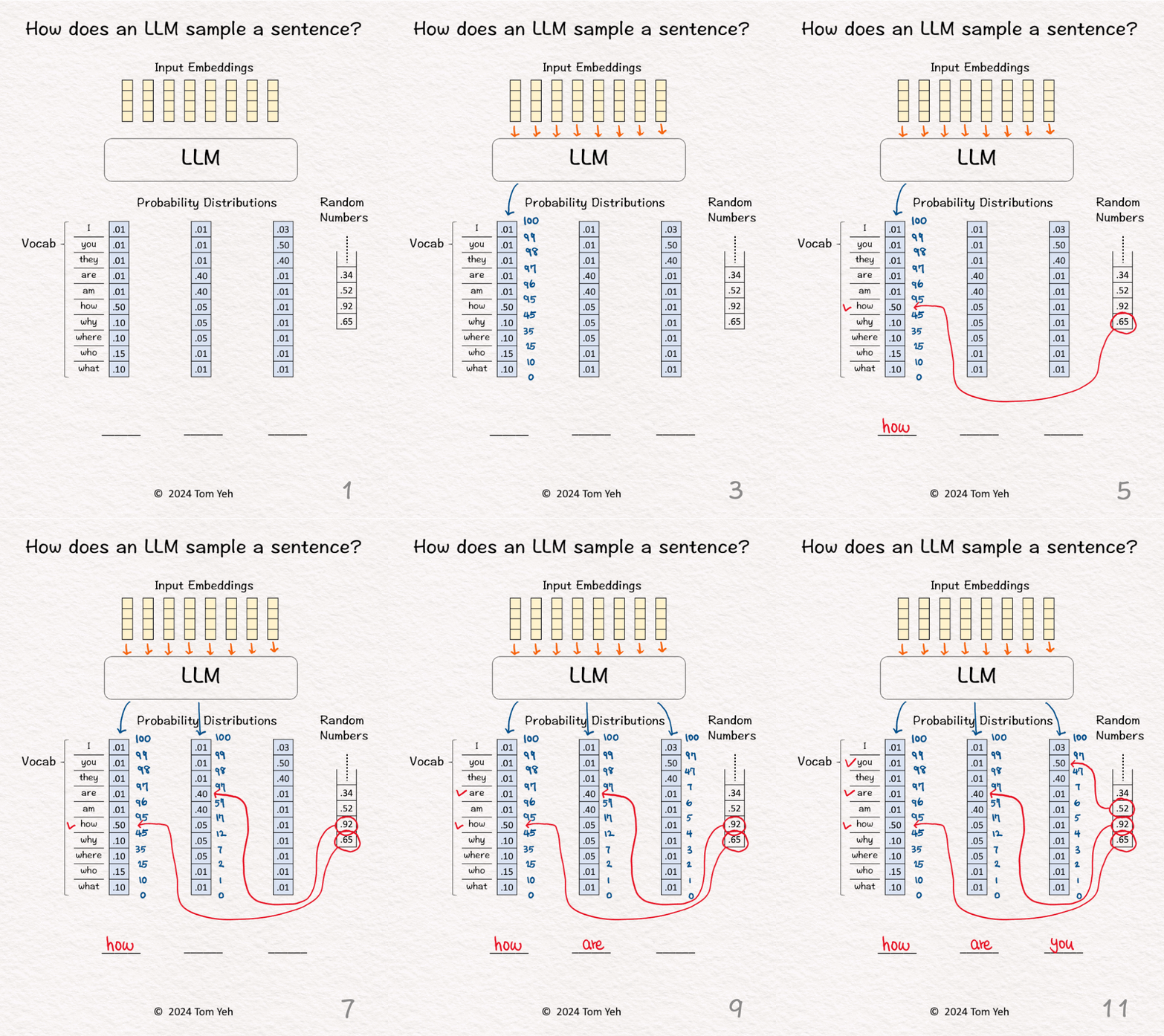
Can you sample a sentence by hand? ✍️
[Like] this post if you can follow the calculation.

In both of my Computer Vision and Generative AI courses, I go into the details of how exactly each pixel in an image or each word in a sentence is sampled from a probability distribution.

The most common visualization of a probability distribution of images or sentences is a cloud. But some students found the cloud representation still too “cloudy.” Thus, I made this hands-on exercise, using concrete numbers to dispel any lingering cloud in their understanding.

— 𝗪𝗮𝗹𝗸𝘁𝗵𝗿𝗼𝘂𝗴𝗵 —

1. Given a sequence of input embeddings, represented as yellow column vectors.
2. Feed the input embeddings to the LLM.
3. The LLM predicts the probability distribution of the next output word over a vocabulary of 10 words, which is represented as a column vector shaded in blue. Then, we calculate the cumulative distribution by hand and write the results in blue. To do so, we start with zero at the bottom, add the number in each cell as we go up, until we reach 100 at the top. Note that for a valid probability distribution, they should add up to 100 (percentage).
4. Draw the next random number (.65) and lookup the range in the cumulative distribution in which this random number falls (.45 < .65 < .95).
5. Lookup the corresponding word (how) and fill that word in the first blank.
6. Repeat step 3 for the next output word
7. Draw the next random number (.92) and lookup the range in the cumulative distribution in which this random number falls (.57 < .92 < .97).
8. Lookup the corresponding word (are) and fill that word in the second blank.
9. Repeat step 3 for the next output word
10. Draw the next random number (.52) and lookup the range in the cumulative distribution in which this random number falls (.47 < .52 < .97).
11. Lookup the corresponding word (you) and fill that word in the third blank.

— 𝗞𝗲𝘆 𝗖𝗼𝗻𝗰𝗲𝗽𝘁𝘀 —

💡 𝗥𝗮𝗻𝗱𝗼𝗺𝗻𝗲𝘀𝘀: The randomness of LLM’s outputs come from a random number generator. To draw a random number is like randomly throwing a dart at a dart board. The outcome is random. The dart will land somewhere. We can’t guarantee where. But we can say it’s likely to land in areas that are larger and less likely to land in areas that are smaller.

💡 𝗗𝗶𝘃𝗲𝗿𝘀𝗶𝘁𝘆: This randomness is what gives diversity to LLM’s outputs.

💡 𝗧𝗲𝗺𝗽𝗲𝗿𝗮𝘁𝘂𝗿𝗲: This hyper-parameter is often used to control the degree of diversity. In this basic exercise, temperature is omitted. Later I will share a more advanced exercise to see the effects of temperature.

💡 𝗜𝗻𝘃𝗲𝗿𝘀𝗲 𝗧𝗿𝗮𝗻𝘀𝗳𝗼𝗿𝗺 𝗦𝗮𝗺𝗽𝗹𝗶𝗻𝗴: If you are familiar with probability theory, you can see this exercise is a simplified version of inverse transform sampling.

POST: https://www.linkedin.com/posts/tom-yeh_deeplearning-pytorch-artificialintelligence-activity-7150130813731287040-zyFe

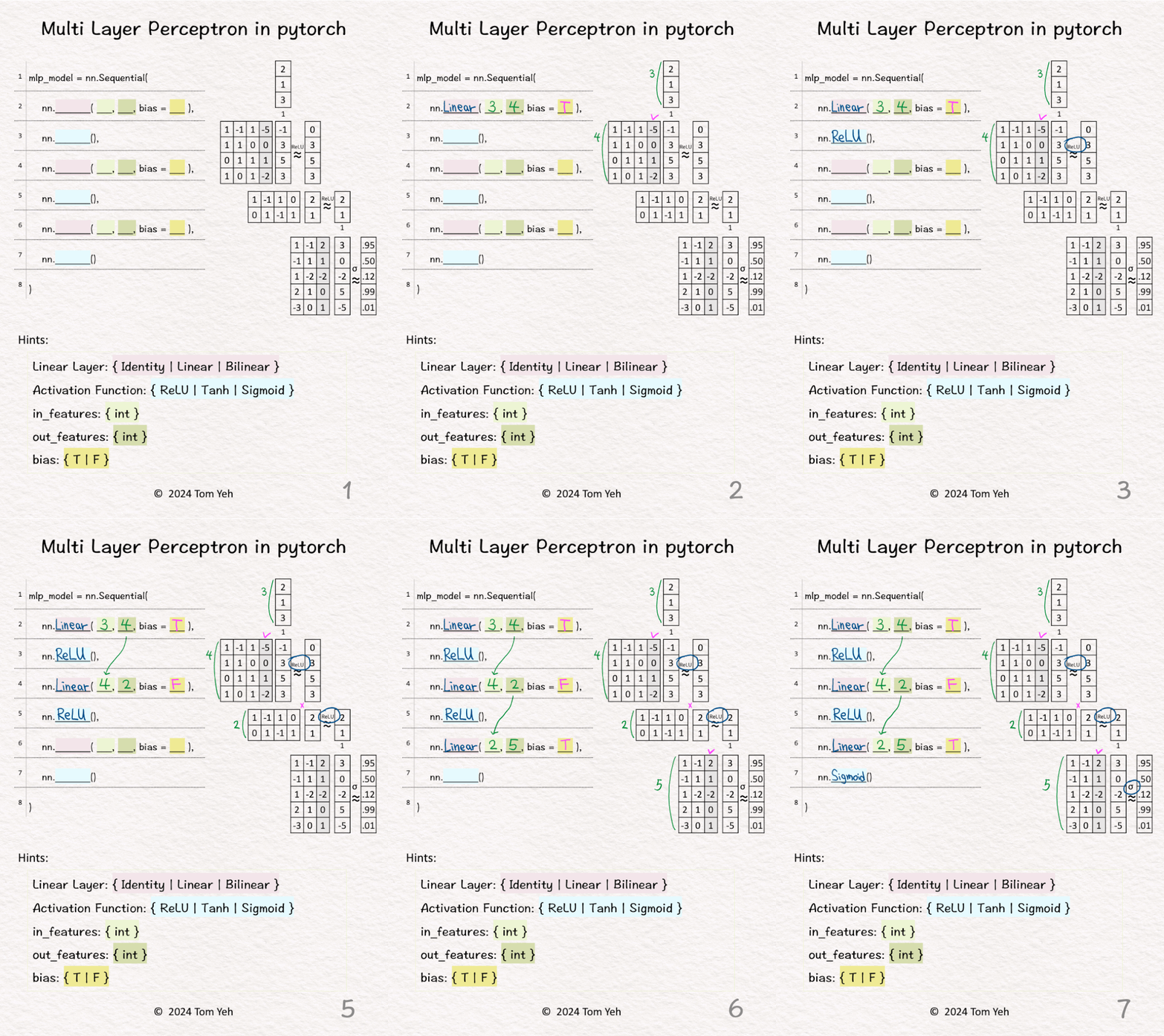
Can you code a multi layer perceptron by hand? ✍️
[Like] this post if you can follow the coding process.

One of the struggles to teach a large course on deep learning is to figure out how to set up a unified coding environment for all the students. Should students use our department’s own cloud infrastructure? Should students use the free Google Colab, Hugging Face, AWS? Should students install the environment in their own laptops (i.e., BYOD)?

Questions like these are important. Without a unified environment, it would be a nightmare for me and my TAs to support the variety of environments students may be using. But, these questions often distract us from the main goal of learning the key programming concepts.

Is it possible go to old-school? Can students practice coding a deep learning framework using pen and paper, but still connecting theories to practices in a meaningful way? It would certainly lower the barrier of entry to learning DL, if we don’t even need computers.

Here’s a hands-on coding exercise I created for this purpose.

— 𝗪𝗮𝗹𝗸𝘁𝗵𝗿𝗼𝘂𝗴𝗵 —

1️⃣ Given a code template (left), implement the multi layer perception as depicted (right).

2️⃣ 𝗙𝗶𝗿𝘀𝘁 𝗹𝗶𝗻𝗲𝗮𝗿 𝗹𝗮𝘆𝗲𝗿. The size of input features is 3. The size of output features is 4. We can see the size of the weight matrix is 4 by 3. Also, there is an extra column for the biases (bias = T).

3️⃣ The activation function is ReLU. We can see the effect of ReLU on the first feature (-1 -> 0).

4️⃣ 𝗦𝗲𝗰𝗼𝗻𝗱 𝗹𝗶𝗻𝗲𝗮𝗿 𝗹𝗮𝘆𝗲𝗿. The size of input features is 4, which is the same as the size of output features from the previous layer. The size of output features is 2. We can see the size of the weight matrix is 2 by 4. But, there isn’t an extra column for the biases (bias = F).

5️⃣ The activation function is ReLU.

6️⃣ 𝗙𝗶𝗻𝗮𝗹 𝗹𝗶𝗻𝗲𝗮𝗿 𝗹𝗮𝘆𝗲𝗿. The size of input features is 2, which is the same as the size of output features from the previous layer. The size of output features is 5. We can see the size of the weight matrix is 5 by 2. Also, there is an extra column for the biases (bias = T).

7️⃣ The activation function is Sigmoid. We can see the effect of Sigmoid, which is a non-linear mapping from raw scores (3, 0, -2, 5, -5) to probability values between 0 and 1.

POST: https://www.linkedin.com/posts/tom-yeh_deeplearning-machinelearning-artificialintelligence-activity-7150568796347363328-LWk0

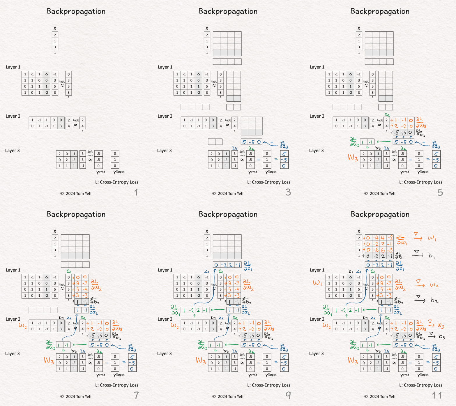
Can you calculate backpropagation of a multi layer perceptron by hand? ✍️
[Like] if you can follow the calculation.

Recently, it has been encouraging to see how the LinkedIn community is embracing my posts about hands-on math for deep learning. I think the audience is ready for a heavy post about backpropagation. 😀

— 𝗪𝗮𝗹𝗸𝘁𝗵𝗿𝗼𝘂𝗴𝗵 —

1. 𝗙𝗼𝗿𝘄𝗮𝗿𝗱 𝗣𝗮𝘀𝘀: Given a multi layer perceptron (3 levels), an input vector X, predictions Y^{Pred} = [0.5, 0.5, 0], and ground truth label Y^{Target} = [0, 1, 0].
2. 𝗕𝗮𝗰𝗸𝗽𝗿𝗼𝗽𝗮𝗴𝗮𝘁𝗶𝗼𝗻: Insert cells to hold our calculations.
3. 𝗟𝗮𝘆𝗲𝗿 𝟯 – 𝗦𝗼𝗳𝘁𝗺𝗮𝘅 (blue): Calculate ∂L / ∂z3 directly using the simple equation: Y^{Pred} – Y^{Target} = [0.5, -0.5, 0]. This simple equation is the benefit of using Softmax and Cross Entropy Loss together.
4. 𝗟𝗮𝘆𝗲𝗿 𝟯 – 𝗪𝗲𝗶𝗴𝗵𝘁𝘀 (orange) & 𝗕𝗶𝗮𝘀𝗲𝘀 (black): Calculate ∂L / ∂W3 and ∂L / ∂b3 by multiplying ∂L / ∂z3 and [ a2 | 1 ].
5. 𝗟𝗮𝘆𝗲𝗿 𝟮 – 𝗔𝗰𝘁𝗶𝘃𝗮𝘁𝗶𝗼𝗻𝘀 (green): Calculate ∂L / ∂a2 by multiplying ∂L / ∂z3 and W3.
6. 𝗟𝗮𝘆𝗲𝗿 𝟮 – 𝗥𝗲𝗟𝗨 (blue): Calculate ∂L / ∂z2 by multiplying ∂L / ∂a2 with 1 for positive values and 0 otherwise.
7. 𝗟𝗮𝘆𝗲𝗿 𝟮 – 𝗪𝗲𝗶𝗴𝗵𝘁𝘀 (orange) & 𝗕𝗶𝗮𝘀𝗲𝘀 (black): Calculate ∂L / ∂W2 and ∂L / ∂b2 by multiplying ∂L / ∂z2 and [ a1 | 1 ].
8. 𝗟𝗮𝘆𝗲𝗿 𝟭 – 𝗔𝗰𝘁𝗶𝘃𝗮𝘁𝗶𝗼𝗻𝘀 (green): Calculate ∂L / ∂a1 by multiplying ∂L / ∂z2 and W2.
9. 𝗟𝗮𝘆𝗲𝗿 𝟭 – 𝗥𝗲𝗟𝗨 (blue): Calculate ∂L / ∂z1 by multiplying ∂L / ∂a1 with 1 for positive values and 0 otherwise.
10. 𝗟𝗮𝘆𝗲𝗿 𝟭 – 𝗪𝗲𝗶𝗴𝗵𝘁𝘀 (orange) & 𝗕𝗶𝗮𝘀𝗲𝘀 (black): Calculate ∂L / ∂W1 and ∂L / ∂b1 by multiplying ∂L / ∂z1 and [ x | 1 ].
11. 𝗚𝗿𝗮𝗱𝗶𝗲𝗻𝘁 𝗗𝗲𝘀𝗰𝗲𝗻𝘁: Update weights and biases (typically a learning rate is applied here).

— 𝗜𝗻𝘀𝗶𝗴𝗵𝘁𝘀 —

💡 𝗠𝗮𝘁𝗿𝗶𝘅 𝗠𝘂𝗹𝘁𝗶𝗽𝗹𝗶𝗰𝗮𝘁𝗶𝗼𝗻 𝗶𝘀 𝗔𝗹𝗹 𝗬𝗼𝘂 𝗡𝗲𝗲𝗱: Just like in the forward pass, backpropagation is all about matrix multiplications. You can definitely do everything by hand as I demonstrated in this exercise, albeit slow and imperfect. This is why GPU’s ability to multiply matrices efficiently plays such an important role in the deep learning evolution. This is why NVIDIA is now close to $1 trillion in valuation.

💡 𝗘𝘅𝗽𝗹𝗼𝗱𝗶𝗻𝗴 𝗚𝗿𝗮𝗱𝗶𝗲𝗻𝘁𝘀: We can already see the gradients are getting larger as we backpropagate up, even in this simple 3-layer network. This motivates using methods like skip connections to handle exploding (or diminishing) gradients as in the ResNet.

POST: https://www.linkedin.com/feed/update/urn:li:share:7151207902123298816/

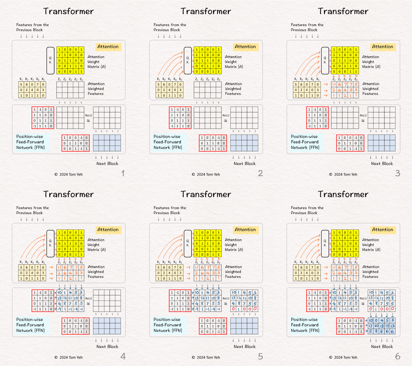
Can you calculate a transformer by hand ✍️?
[Like] if you can follow the calculation.

To study the transformer architecture, it is like opening up the hood of a car and seeing all sorts of engine parts: embeddings, positional encoding, feed-forward network, attention weighting, self-attention, cross-attention, multi-head attention, layer norm, skip connections, softmax, linear, Nx, shifted right, query, key, value, masking. This list of jargons feels overwhelming!

What are the key parts that really make the transformer (🚗) run?

In my opinion, the 🔑 key is the combination of: [attention weighting] and [feed-forward network].

All the other parts are enhancements to make the transformer (🚗) run faster and longer, which is still important because those enhancements are what lead us to “large” language models. 🚗 -> 🚚

— 𝗪𝗮𝗹𝗸𝘁𝗵𝗿𝗼𝘂𝗴𝗵 —

[1] Given
↳ Input features from the previous block (5 positions)

[2] Attention
↳ Feed all 5 features to a query-key attention module (QK) to obtain an attention weight matrix (A). I will skip the details of this module. In a follow-up post I will unpack this module.

[3] Attention Weighting
↳ Multiply the input features with the attention weight matrix to obtain attention weighted features (Z). Note that there are still 5 positions.
↳ The effect is to combine features a͟c͟r͟o͟s͟s͟ ͟p͟o͟s͟i͟t͟i͟o͟n͟s͟ (horizontally), in this case, X1 := X1 + X2, X2 := X2 + X3….etc.

[4] FFN: First Layer
↳ Feed all 5 attention weighted features into the first layer.
↳ Multiply these features with the weights and biases.
↳ The effect is to combine features a͟c͟r͟o͟s͟s͟ ͟f͟e͟a͟t͟u͟r͟e͟ ͟d͟i͟m͟e͟n͟s͟i͟o͟n͟s͟ (vertically).
↳ The dimensionality of each feature is increased from 3 to 4.
↳ Note that each position is processed by the same weight matrix. This is what the term “position-wise” is referring to.
↳ Note that the FFN is essentially a multi layer perceptron.

[5] ReLU
↳ Negative values are set to zeros by ReLU.

[6] FFN: Second Layer
↳ Feed all 5 features (d=3) into the second layer.
↳ The dimensionality of each feature is decreased from 4 back to 3.
↳ The output is fed to the next block to repeat this process.
↳ Note that the next block would have a completely separate set of parameters.

Together, the two key parts: attention and FFN, transform features both across positions and across feature dimensions. This is what makes the transformer (🚗) run!

POST: https://www.linkedin.com/posts/tom-yeh_deeplearning-neuralnetworks-datascience-activity-7152297663122554880-p550

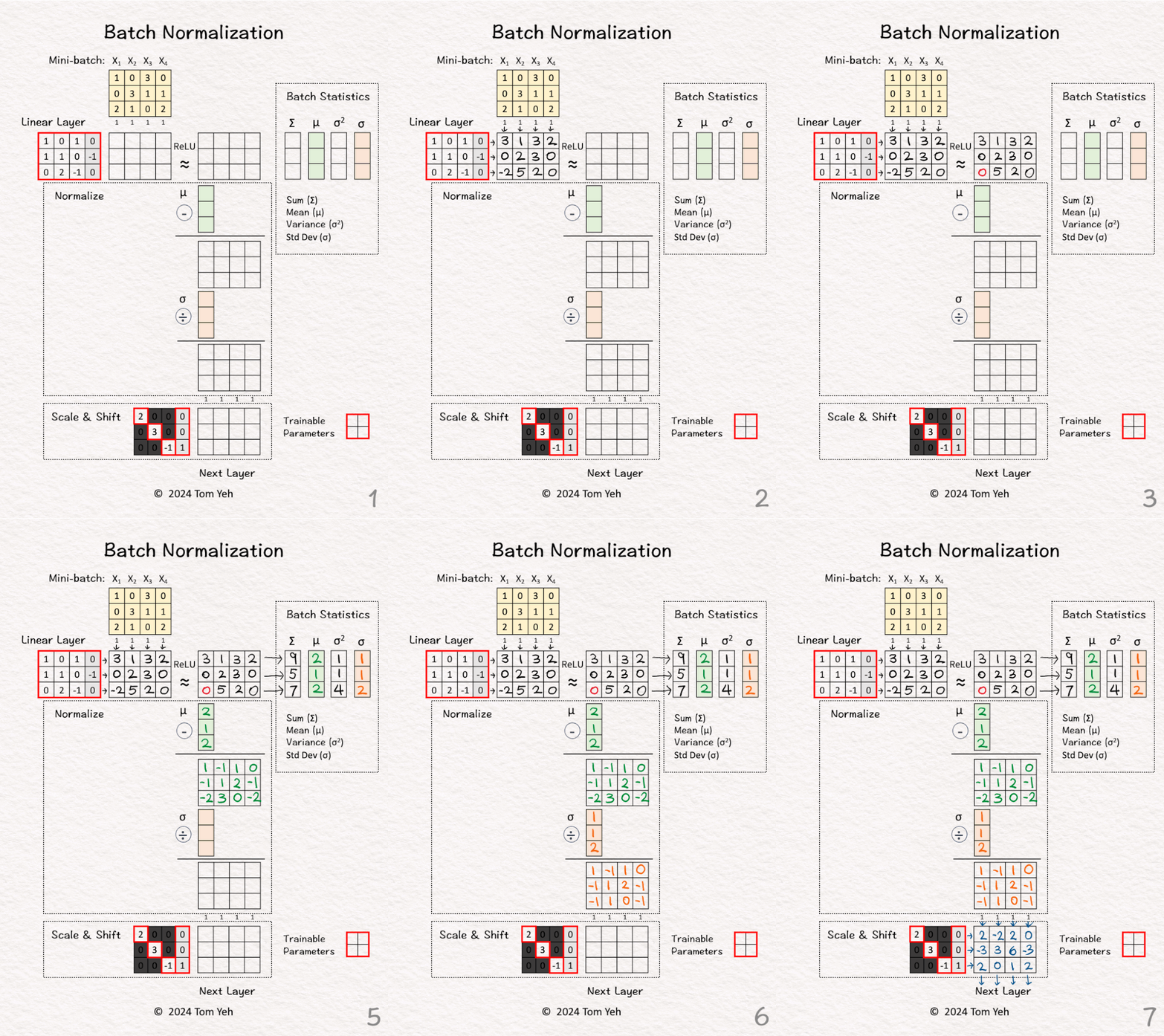
Can you calculate batch normalization by hand? ✍️
[Like] if you can follow the calculation.

Batch normalization is a common practice to improve training and achieve faster convergence. It sounds simple. But it is often misunderstood.

🤔 Does batch normalization involve trainable parameters? tunable hyper-parameters? or both?

🤔 Is batch normalization applied to inputs, features, weights, biases, or outputs?

🤔 How is batch normalization different from layer normalization?

This hands-on exercise can help shed some light on these questions.

— 𝗪𝗮𝗹𝗸𝘁𝗵𝗿𝗼𝘂𝗴𝗵 —

[1] Given
↳ A mini-batch of 4 training examples, each has 3 features.

[2] Linear Layer
↳ Multiply with the weights and biases to obtain new features

[3] ReLU
↳ Apply the ReLU activation function, which has the effect of suppressing negative values. In this exercise, -2 is set to 0.

[4] Batch Statistics
↳ Compute the sum, mean, variance, and standard deviation across the four examples in this min-batch.
↳ Note that these statistics are computed for each row (i.e., each feature dimension).

[5] Shift to Mean = 0
↳ Subtract the mean (green) from the activation values for each training example
↳ The intended effect is for the 4 activation values in each dimension to average to zero

[6] Scale to Variance = 1
↳ Divide by the standard deviation (orange)
↳ The intended effect is for the 4 activation values to have variance equal to one.

[7] Scale & Shift
↳ Multiply the normalized features from [6] by a linear transformation matrix, and pass the results to the next layer
↳ The intended effect is to scale and shift the normalized feature values to a new mean and variance, which are to be learned by the network
↳ The elements in the diagonal and the last column are trainable parameters the network will learn.

POST: https://www.linkedin.com/posts/tom-yeh_deeplearning-gan-artificialintelligence-activity-7152664087968055296-1AJb

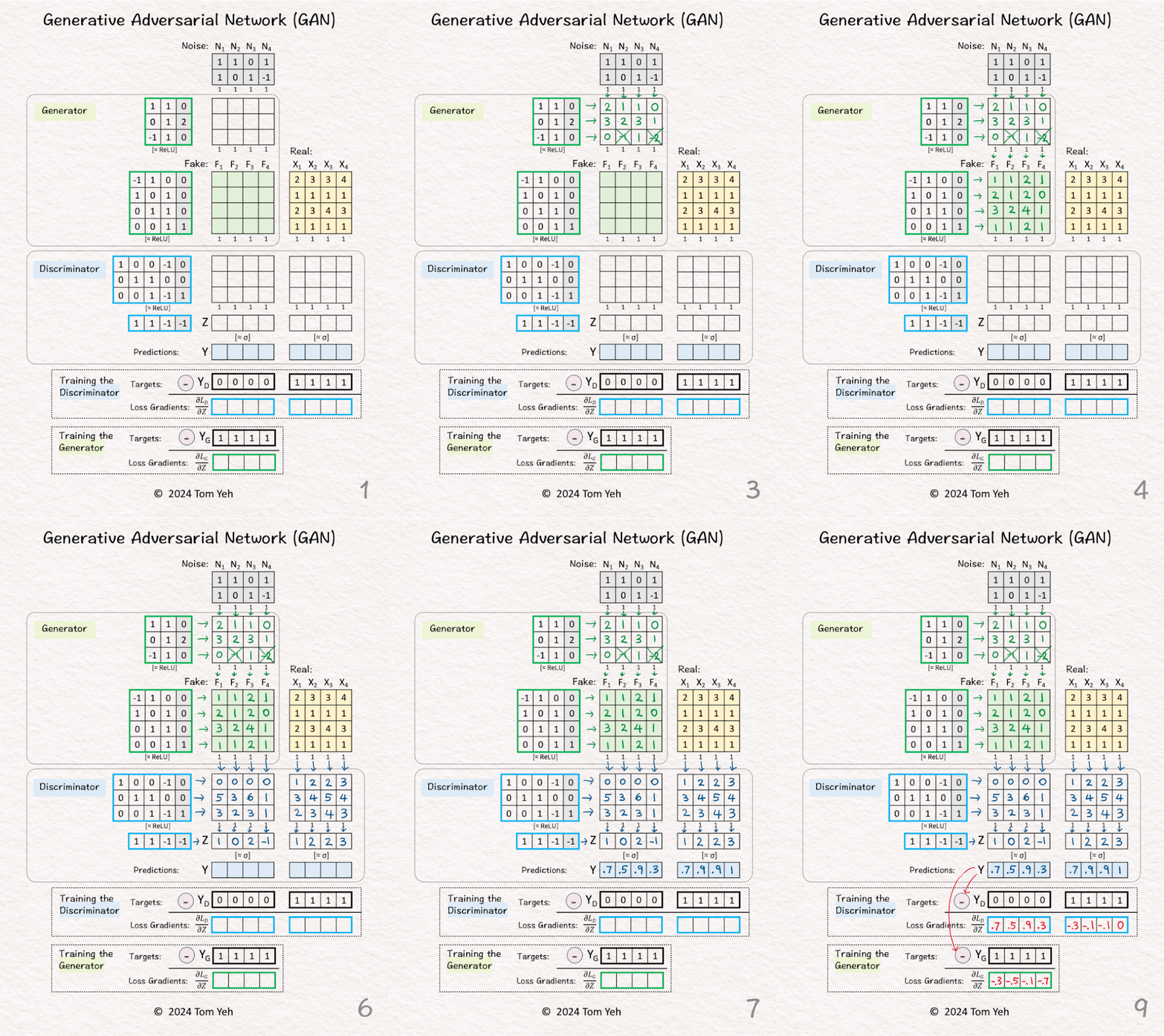
Can you calculate a generative adversarial network (GAN) by hand? ✍️
[Like] if you can follow the calculation.

GANs need no introduction. Invented by Ian Goodfellow in 2014, GANs are responsible for starting the field of Generative AI for visual data.

— 𝗪𝗮𝗹𝗸𝘁𝗵𝗿𝗼𝘂𝗴𝗵 —

𝗚𝗼𝗮𝗹: Generate realistic 4-D data from 2-D noise.

[1] Given
↳ 4 noise vectors in 2D (N)
↳ 4 real data vectors in 4D (X)

[2] 🟩 Generator: First Layer
↳ Multiply the noise vectors with weights and biases to obtain new feature vectors

[3] 🟩 Generator: ReLU
↳ Apply the ReLU activation function, which has the effect of suppressing negative values. In this exercise, -1 and -2 are crossed out and set to 0.

[4] 🟩 Generator: Second Layer
↳ Multiply the features with weights and biases to obtain new feature vectors.
↳ ReLU is applied. But since every value is positive, there’s no effect.
↳ These new feature vectors are the “Fake” data (F) generated by this simple 2-layer Generator network.

[5] 🟦 Discriminator: First Layer
↳ Feed both Fake data (F) and real data (X) to the first linear layer
↳ Multiply F and X with weights and biases to obtain new feature vectors.
↳ ReLU is applied. But since every value is positive, there’s no effect.

[6] 🟦 Discriminator: Second Layer
↳ Multiply the features with one set of weights and bias to obtain new features.
↳ The intended effect is to reduce to just one feature value per data vector.

[7] 🟦 Discriminator: Sigmoid σ
↳ Convert features (Z) to probability values (Y) using the Sigmoid function
↳ 1 means the Discriminator is 100% confident the data is real.
↳ 0 means the Discriminator is 100% confident the data is fake.

[8] 🏋️ Training: 🟦 Discriminator
↳ Compute the loss gradients of the Discriminator by the simple equation of Y – YD. Why so simple? Because when we use sigmoid and binary entropy loss together, the math magically simplifies to this equation.
↳ YD are the target predictions from the Discriminator’s perspective. The Discriminator must learn to predict 0 for the four Fake data (F) and 1 for the four Real data (X). YD=[0,0,0,0,1,1,1,1].
↳ Note that the Discriminator’s loss involves both the Fake data and Real data.
↳ With the loss gradients computed, we can kickoff the back propagation process to update the Discriminator’s weights and biases (blue borders).

[9] 🏋️ Training: 🟩 Generator
↳ Compute the loss gradients of the Generator by the simple equation of Y – YG.
↳ YG are the target predictions from the Generator’s perspective. The Generator must fool the Discriminator into predicting 1 for the four Fake data (F). YG=[1,1,1,1].
↳ Note that the Generator’s loss involves only the Fake data.
↳ With the loss gradients computed, we can kickoff the back propagation process to update the Generator’s weights and biases (green borders).

POST: https://www.linkedin.com/feed/update/urn:li:share:7153234214803357697/

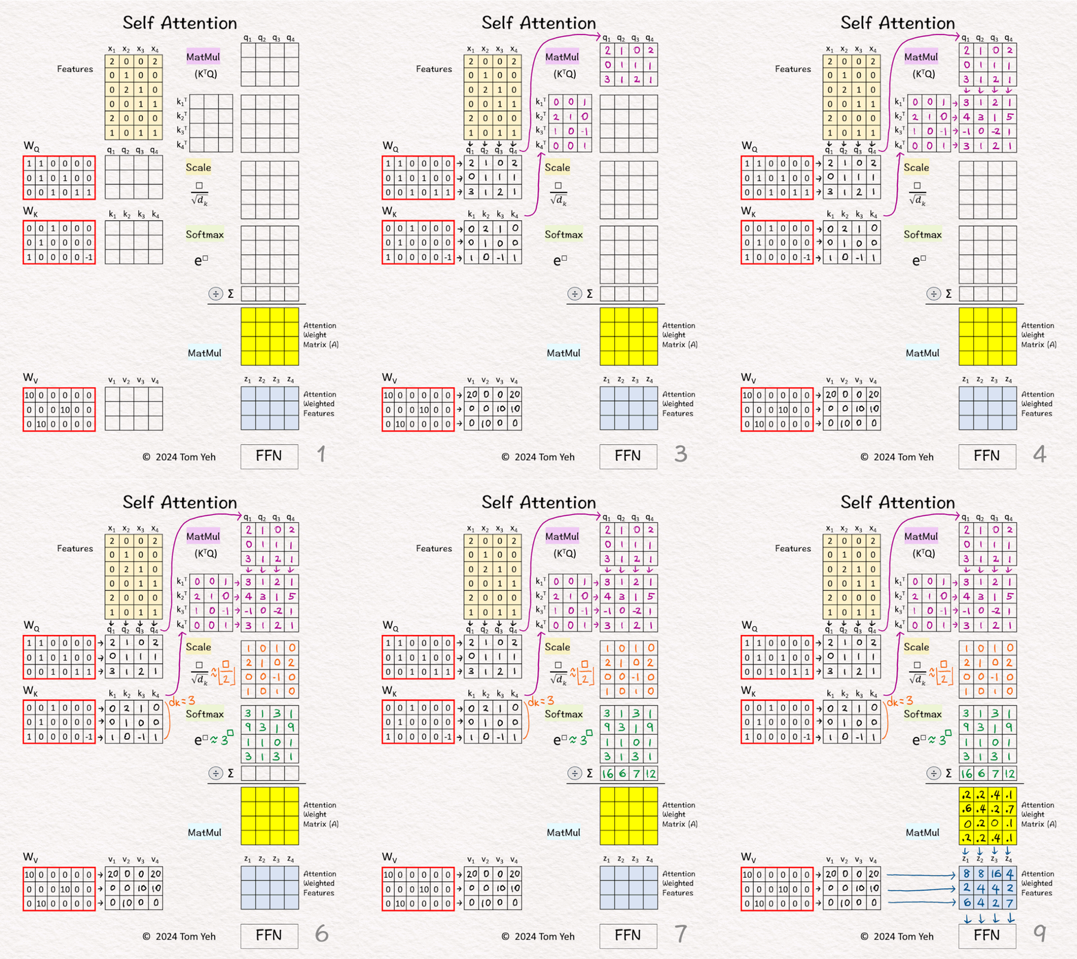
Can you calculate self attention by hand? ✍️
[Like] if you can follow the calculation.

— 𝗚𝗼𝗮𝗹  —

Features (6-D) (orange) –> Attention Weighted Features (3-D) (blue)

— 𝗪𝗮𝗹𝗸𝘁𝗵𝗿𝗼𝘂𝗴𝗵 —

[1] Given
↳ A set of 4 feature vectors (6-D)

[2] Query, Key, Value
↳ Multiply features x’s with linear transformation matrices WQ, WK, and WV, to obtain query vectors (q1,q2,q3,q4), key vectors (k1,k2,k3,k4), and value vectors (v1,v2,v3,v4).
↳ “Self” refers to the fact that both queries and keys are derived from the same set of features.

[3] 🟪 Prepare for MatMul
↳ Copy query vectors
↳ Copy the transpose of key vectors

[4] 🟪 MatMul
↳ Multiply K^T and Q
↳ This is equivalent to taking dot product between every pair of query and key vectors.
↳ The purpose is to use dot product as an estimate of the “matching score” between every key-value pair.
↳ This estimate makes sense because dot product is the numerator of Cosine Similarity between two vectors.

[5] 🟨 Scale
↳ Scale each element by the square root of dk, which is the dimension of key vectors (dk=3).
↳ The purpose is to normalize the impact of the dk on matching scores, even if we scale dk to 32, 64, or 128.
↳ To simplify hand calculation, we approximate [ □/sqrt(3) ] with [ floor(□/2) ].

[6] 🟩 Softmax: e^x
↳ Raise e to the power of the number in each cell
↳ To simplify hand calculation, we approximate e^□ with 3^□.

[7] 🟩 Softmax: ∑
↳ Sum across each column

[8] 🟩 Softmax: 1 / sum
↳ For each column, divide each element by the column sum
↳ The purpose is normalize each column so that the numbers sum to 1. In other words, each column is a probability distribution of attention, and we have four of them.
↳ The result is the Attention Weight Matrix (A) (yellow)

[9] 🟦 MatMul
↳ Multiply the value vectors (Vs) with the Attention Weight Matrix (A)
↳ The results are the attention weighted features Zs.
↳ They are fed to the position-wise feed forward network in the next layer.

POST: https://www.linkedin.com/posts/tom-yeh_deeplearning-datascience-algorithm-activity-7154270359649710080-UjNV

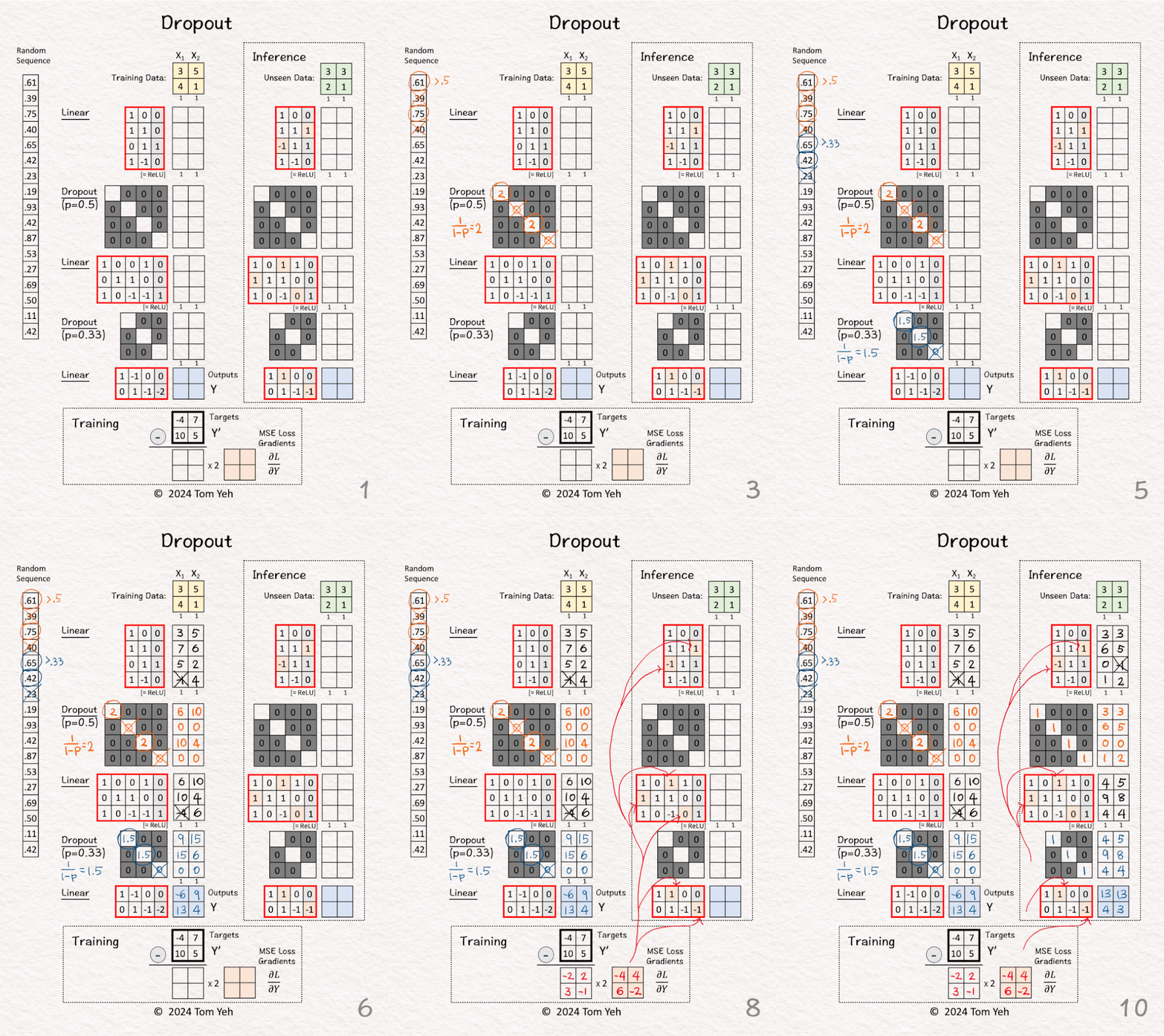
 Can you calculate dropout by hand? ✍️
[Like] if you can follow the calculation.

Dropout is a simple yet effective way of reducing overfitting and improving generalization. This hands-on exercise lets students practice calculating dropout, thereby gaining insight into its inner workings.

As an additional bonus, students get to practice calculating the gradients of the Mean Square Error (MSE) loss. After the practice, students are often surprised by how simple it is.

— 𝗡𝗲𝘁𝘄𝗼𝗿𝗸 𝗔𝗿𝗰𝗵𝗶𝘁𝗲𝗰𝘁𝘂𝗿𝗲 —

1. Linear(2,4)
2. ReLU
3. Dropout(0.5)
4. Linear(4,3)
5. ReLU
6. Dropout(0.33)
7. Linear(3,2)

— 𝗪𝗮𝗹𝗸𝘁𝗵𝗿𝗼𝘂𝗴𝗵 —

🏋️ Training

[1] Given
↳ A  training set of 2 examples X1, X2

[2] 🟧 Random: p > 0.5
↳ Draw 4 random numbers
↳ For each random number, if it is above 0.5, we keep and denote it as ◯. Otherwise we drop and denote it as ╳.
↳ The result is [◯, ╳, ◯, ╳]

[3] 🟧 Dropout: Matrix
↳ Calculate the scaling factor: 1 / (1-p) = 2
↳ Set the diagonal based on [◯, ╳, ◯, ╳], where ◯ = 2 and  ╳ = 0
↳ The purpose is to drop the 2nd and the 4th nodes, and scale the remaining two nodes by 2.

[4] 🟦 Random: p > 0.33
↳ Draw 3 random numbers
↳ For each random number, if it is above 0.33, we keep and denote it as ◯. Otherwise we drop and denote it as ╳.
↳ The result is [◯, ◯, ╳]

[5] 🟦 Dropout: Matrix
↳ Calculate the scaling factor: 1 / (1-p) = 1.5
↳ Set the diagonal based on [◯, ◯, ╳], where ◯ = 1.5 and  ╳ = 0
↳ The purpose is to drop the 3rd node, and scale the remaining two nodes by 1.5.

[6] Feed Forward
↳ Now we have all the matrices ready across the layers, perform the feed forward pass by calculating a series of matrix multiplications from the top to the bottom
↳ ReLU activation function is applied along the way to set negative feature values to zeroes, denoted by ╳.
↳ The outputs are Y.

[7] 🟥 Loss Gradients of Mean Square Error (MSE)
↳ The formula is 2 * (Y – Y’)
↳ First we calculate Outputs (Y) – Targets (Y’)
↳ Second we multiply each element by 2

[8] Update Weights
↳ Use loss gradients to start back propagation
↳ Update some weights (light red)
↳ The values of the new weights are for demonstration purpose only, not based on real calculation.

🔍 Inference

[9] Deactivate Dropout
↳ We set both dropout matrices to identity matrices
↳ The effect is to keep all the features as is.

[10] Feed Forward
↳ Take the forward pass to make predictions about unseen data.

POST: https://www.linkedin.com/posts/tom-yeh_deeplearning-algorithm-neuralnetwork-activity-7155188284233601024-TJwt

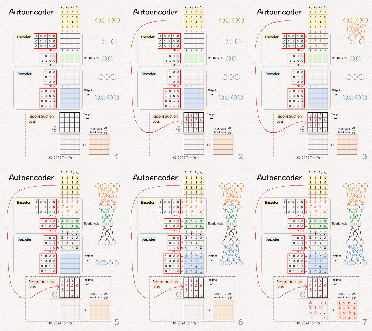
Can you calculate an autoencoder by hand? ✍️
[Like] if you can follow the calculation.

The autoencoder model is the basis for training foundational models from a ton of data. We are talking about tens of billions of training examples, like a good portion of the Internet.

With that much data, it is not economically feasible to hire humans to label all of those data to tell a model what its targets are. Thus, people came up with many clever ideas to derive training targets from the training examples themselves [auto]matically.

The most straightforward idea is to just use the training data itself as the targets. This hands-on exercise demonstrates this idea.

Then, people tried hiding some parts of the training data and using those missing parts as the targets. This is called masking, which is how LLMs are trained these days.

Then, people tried pairing up text and images and using each other as targets. This is called “constrative” learning. This is the C in the famous CLIP model from OpenAI, which is the basis of all the multimodal foundational models.

Let’s start with the basic—autoencoder.

— 𝗡𝗲𝘁𝘄𝗼𝗿𝗸 𝗔𝗿𝗰𝗵𝗶𝘁𝗲𝗰𝘁𝘂𝗿𝗲 —

🟨 Encoder
1. Linear(4,3)
2. ReLU
3. Linear(3,2)
4. ReLU

🟦 Decoder
1. Linear(2,3)
2. ReLU
3. Linear(3,4)

— 𝗪𝗮𝗹𝗸𝘁𝗵𝗿𝗼𝘂𝗴𝗵 —

[1] Given
↳ Four training examples X1, X2, X3, X4

[2] Auto
↳ Copy training examples to Targets (Y’)
↳ The purpose is to train the network to reconstruct the training examples.
↳ Since each target is a training example itself, we use the Greek word “auto” which means “self.” This crucial step is what makes an autoencoder “auto.”

[3] 🟨 Encoder: Layer 1 + ReLU
↳ Multiply inputs with weights and biases
↳Apply ReLU, crossing out negative values (-1 -> 0)

[4] 🟨 Encoder: Layer 2 + ReLU
↳ Multiply features with weights and biases
↳Apply ReLU, crossing out negative values (-1 -> 0)
↳ This layer is often called the “bottleneck” because its outputs (green 🟩) have a lot fewer feature dimensions (2) than the input features (4).

[5] 🟦 Decoder: Layer 1 + ReLU
↳ Multiply features with weights and biases
↳ Apply ReLU, crossing out negative values. Here, no negative values to cross out.

[6] 🟦 Decoder: Layer 2
↳ Multiply features with weights and biases
↳ The Outputs (Y) are the Decoder’s attempt to reconstruct the training examples from their reduced 2-D representation (green 🟩).

[7] 🟥 Loss Gradients & Backpropagation
↳ Calculate the gradients of the Mean Square Error (MSE) loss between the outputs (Y) and targets (Y’).
↳ The formula is 2 * (Y – Y’)
↳ First we calculate Outputs (Y) – Targets (Y’)
↳ Second we multiply each element by 2
↳ These gradients kick off the backpropagation process to update weights and biases.

POST: https://www.linkedin.com/posts/tom-yeh_vectordatabase-rag-deeplearning-activity-7158816842730336257-BaSm

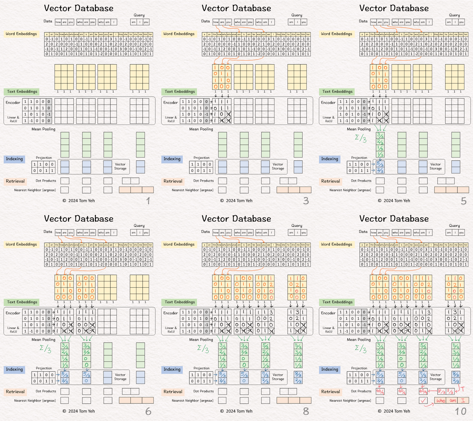
Can you calculate a vector database by hand? ✍️
[Like] if you can follow the calculation.

Vector databases are revolutionizing how we search and analyze complex data. They have become the backbone of Retrieval Augmented Generation (RAG).

How do vector databases work?

[1] Given
↳ A dataset of three sentences, each has 3 words (or tokens)
↳ In practice, a dataset may contain millions or billions of sentences. The max number of tokens may be tens of thousands (e.g., 32,768 mistral-7b).

Process “how are you”

[2] 🟨 Word Embeddings
↳ For each word, look up corresponding word embedding vector from a table of 22 vectors, where 22 is the vocabulary size.
↳ In practice, the vocabulary size can be tens of thousands. The word embedding dimensions are in the thousands (e.g., 1024, 4096)

[3] 🟩 Encoding
↳ Feed the sequence of word embeddings to an encoder to obtain a sequence of feature vectors, one per word.
↳ Here, the encoder is a simple one layer perceptron (linear layer + ReLU)
↳ In practice, the encoder is a transformer or one of its many variants.

[4] 🟩 Mean Pooling
↳ Merge the sequence of feature vectors into a single vector using “mean pooling” which is to average across the columns.
↳ The result is a single vector. We often call it “text embeddings” or “sentence embeddings.”
↳ Other pooling techniques are possible, such as CLS. But mean pooling is the most common.

[5] 🟦 Indexing
↳ Reduce the dimensions of the text embedding vector by a projection matrix. The reduction rate is 50% (4->2).
↳ In practice, the values in this projection matrix is much more random.
↳ The purpose is similar to that of hashing, which is to obtain a short representation to allow faster comparison and retrieval.
↳ The resulting dimension-reduced index vector is saved in the vector storage.

[6] Process “who are you”
↳ Repeat [2]-[5]

[7] Process “who am I”
↳ Repeat [2]-[5]

Now we have indexed our dataset in the vector database.

[8] 🟥 Query: “am I you”
↳ Repeat [2]-[5]
↳ The result is a 2-d query vector.

[9] 🟥 Dot Products
↳ Take dot product between the query vector and database vectors. They are all 2-d.
↳ The purpose is to use dot product to estimate similarity.
↳  By transposing the query vector, this step becomes a matrix multiplication.

[10] 🟥 Nearest Neighbor
↳ Find the largest dot product by linear scan.
↳ The sentence with the highest dot product is “who am I”
↳ In practice, because scanning billions of vectors is slow, we use an Approximate Nearest Neighbor (ANN) algorithm like the Hierarchical Navigable Small Worlds (HNSW).

Daniel Svonava, co-founder of Superlinked, generously lent his immense knowledge about vector databases to me by reviewing a draft of this post and providing valuable feedback. Follow him to learn more about vector databases.

POST: https://www.linkedin.com/posts/tom-yeh_deeplearning-algorithm-neuralnetwork-activity-7162252913388535808-CbO2

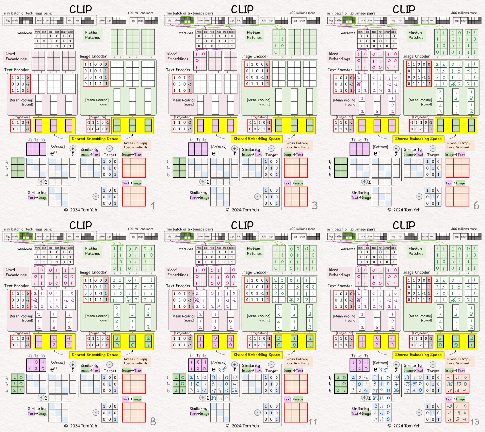
Can you calculate CLIP by hand? ✍️
[Like] if you can follow the calculation.

The CLIP (Contrastive Language–Image Pre-training) model, a groundbreaking work by OpenAI, redefines the intersection of computer vision and natural language processing. It is the basis of all the multi-modal foundation models we see today.

How does CLIP work?

— 𝗚𝗼𝗮𝗹 —

🟨 Learn a shared embedding space for text and image

— 𝗪𝗮𝗹𝗸𝘁𝗵𝗿𝗼𝘂𝗴𝗵 —

[1] Given
↳ A mini batch of 3 text-image pairs
↳ OpenAI used 400 million text-image pairs to train its original CLIP model.

Process 1st pair: “big table”

[2] 🟪 Text → 2 Vectors (3D)
↳ Look up word embedding vectors using word2vec.

[3] 🟩 Image → 2 Vectors (4D)
↳ Divide the image into two patches.
↳ Flatten each patch

[4] Process other pairs
↳ Repeat [2]-[3]

[5] 🟪 Text Encoder & 🟩 Image Encoder
↳ Encode input vectors into feature vectors
↳ Here, both encoders are simple one layer perceptron (linear + ReLU)
↳ In practice, the encoders are usually transformer models.

[6] 🟪 🟩  Mean Pooling: 2 → 1 vector
↳ Average 2 feature vectors into a single vector by averaging across the columns
↳ The goal is to have one vector to represent each image or text

[7] 🟪 🟩 -> 🟨 Projection
↳ Note that the text and image feature vectors from the encoders have different dimensions (3D vs. 4D).
↳ Use a linear layer to project image and text vectors to a 2D shared embedding space.

🏋️ Contrastive Pre-training 🏋️

[8] Prepare for MatMul
↳ Copy text vectors (T1,T2,T3)
↳ Copy the transpose of image vectors (I1,I2,I3)
↳ They are all in the 2D shared embedding space.

[9] 🟦 MatMul
↳ Multiply T and I matrices.
↳ This is equivalent to taking dot product between every pair of image and text vectors.
↳ The purpose is to use dot product to estimate the similarity between a pair of image-text.

[10] 🟦 Softmax: e^x
↳ Raise e to the power of the number in each cell
↳ To simplify hand calculation, we approximate e^□ with 3^□.

[11] 🟦 Softmax: ∑
↳ Sum each row for  🟩 image→🟪 text
↳ Sum each column for 🟪 text→ 🟩 image

[12] 🟦 Softmax: 1 / sum
↳ Divide each element by the column sum to obtain a similarity matrix for 🟪 text→🟩 image
↳ Divide each element by the row sum to obtain a similarity matrix for 🟩 image→🟪 text

[13] 🟥 Loss Gradients
↳ The “Targets” for the similarity matrices are Identity Matrices.
↳ Why? If I and T come from the same pair (i=j), we want the highest value, which is 1, and 0 otherwise.
↳ Apply the simple equation of [Similarity – Target] to compute gradients of for both directions.
↳ Why so simple? Because when Softmax and Cross-Entropy Loss are used together, the math magically works out that way.
↳ These gradients kick off the backpropagation process to update weights and biases of the encoders and projection layers (red borders).

POST: https://www.linkedin.com/posts/tom-yeh_deeplearning-algorithm-neuralnetwork-activity-7163898331201482753-lt6C

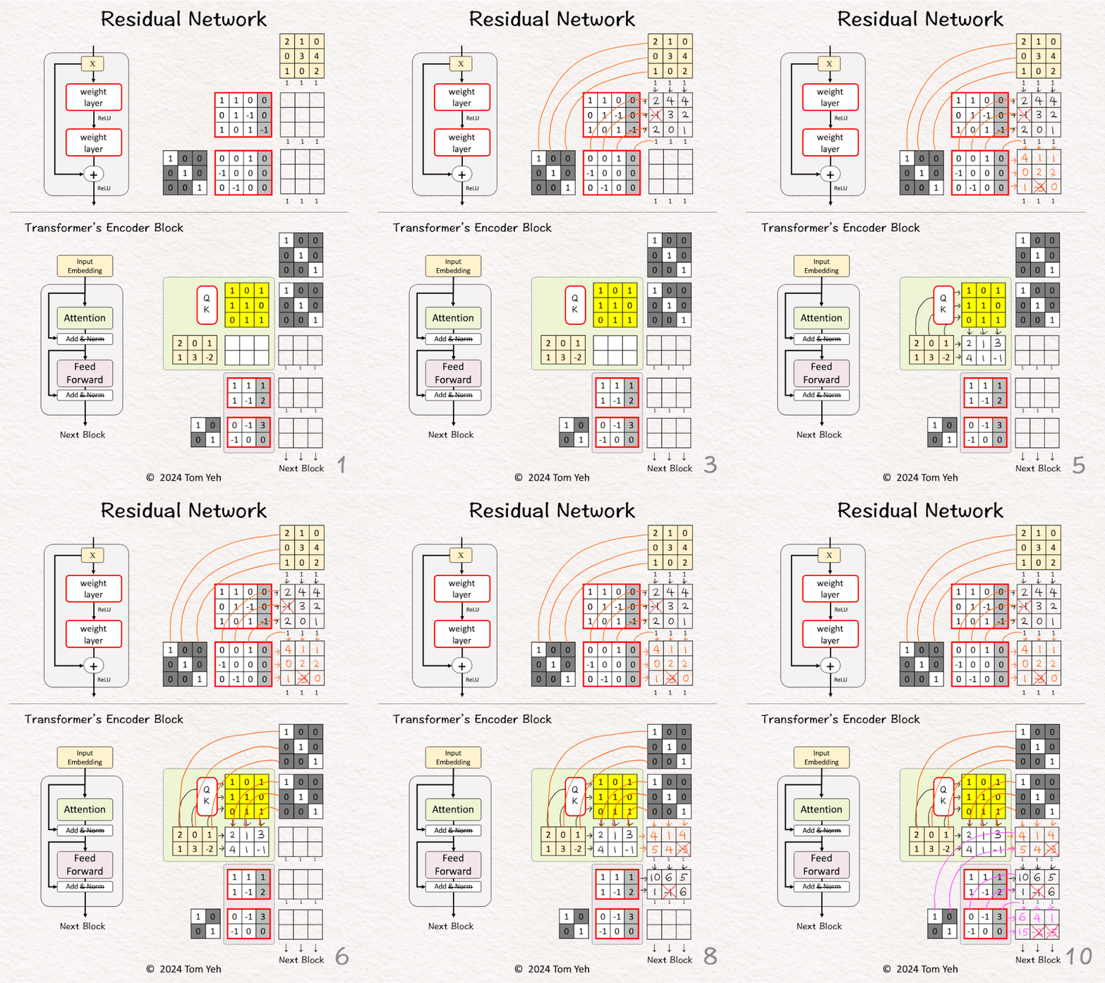
Can you calculate ResNet by hand? ✍️
[Like] if you can follow the calculation.

The most cited deep learning paper ever (>200K), yet often hidden from the public’s eyes, is “Deep Residual Learning for Image Recognition” published by Kaiming He in CVPR 2016.

To put 200K citations in context, CVPR accepts 2000 papers on average. It will take 100 years for every single accepted paper in CVPR to cite this paper to get to 200K citations.

Wow!

Why is ResNet so important?

Because it found a simple solution to solve the exploding and diminishing gradient problems of deep neural networks. It made 10,000’s layers possible.

How simple is this solution?

An identify matrix!

— 𝗪𝗮𝗹𝗸𝘁𝗵𝗿𝗼𝘂𝗴𝗵 —

R͟e͟s͟i͟d͟u͟a͟l͟ ͟B͟l͟o͟c͟k͟

[1] Given
↳ A mini batch of 3 input vectors (3D)

[2] Linear Layer
↳ Multiply the input with weights and bias
↳ Apply ReLU (negatives → 0)
↳ Obtain 3 feature vectors

[3] Concatenate
↳ Stack (horizontally) an identity matrix and the weight and bias matrix of the 2nd layer
↳ Stack (vertically) the input vectors and the feature vectors from the previous layer
↳ Draw lines to visualize the links between rows (weights) and columns (features)
↳ These links are the “Skip Connections”

[4] Linear Layer + Identity
↳ Multiply the two stacked matrices
↳ This is equivalent to F(X) + X
↳ Apply ReLU (negatives → 0)
↳ Pass the results to the next residual block

T͟r͟a͟n͟s͟f͟o͟r͟m͟e͟r͟’͟s͟ ͟E͟n͟c͟o͟d͟e͟r͟ ͟B͟l͟o͟c͟k͟

Let’s see how residual block (aka. skip connections) work in a transformer model

[5] 🟩 Attention
↳ A sequence of 3 input vectors (2D)
↳ Compute an attention matrix (bright yellow)
↳ Multiply the input vectors with the attention matrix to obtain attention-weighted vectors.
↳ Read [Self Attention by hand  ✍️ ] https://lnkd.in/gDW8Um4W to learn more.

[6] 🟩 Concatenate
↳ Stack two identity matrices (to achieve 1 + 1)
↳ Stack the input vectors and the attention-weighted vectors
↳ Draw skip connections

[7] 🟩 Add
↳ Multiply the two stacked matrices

[8] 🟪 Feed Forward: First Layer
↳ Multiply the input with weights and bias
↳ Apply ReLU (negatives → 0)
↳ Obtain 3 feature vectors

[9] 🟪 Feed Forward: Concatenate
↳ Stack and visualize like step [3]

[10] 🟪 Feed Forward: Second Layer + Identity
↳ Multiply the two stacked matrices
↳ Apply ReLU (negatives → 0)
↳ Pass the results to the next encoder block

Did you notice that sizes and positions of the identity matrices are different?

This difference illustrates the magic of the transformer block:
• The attention layer combines positions (across columns)
• The feed forward layer combines features (across rows)
Read the [Transformer by hand  ✍️ ] https://lnkd.in/g39jcD7j to learn more.

POST: https://www.linkedin.com/posts/tom-yeh_deeplearning-algorithm-neuralnetwork-activity-7164629532249894912-RBSZ

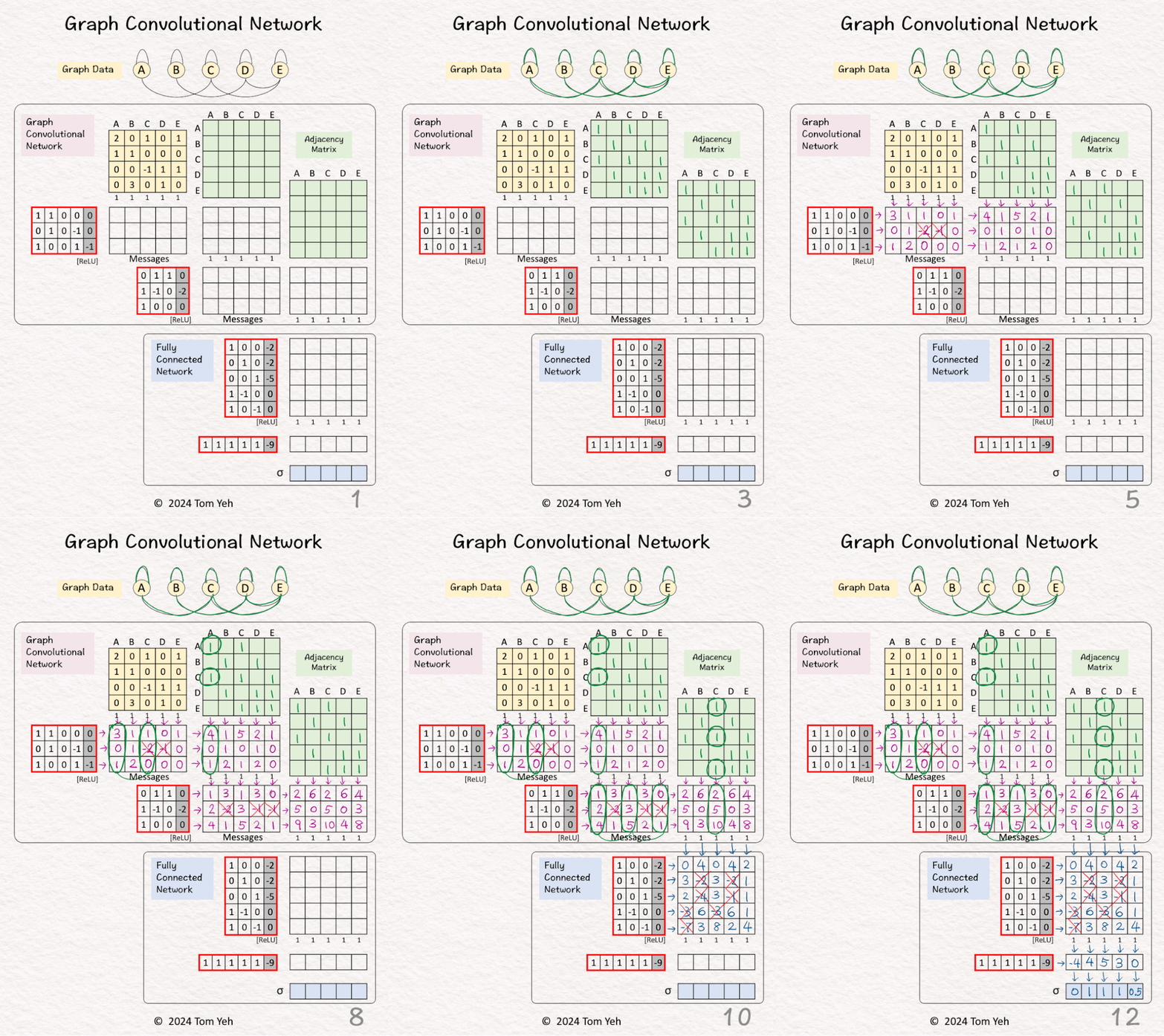
 Can you calculate a Graph Convolutional Network (GCN) by hand? ✍️
[Like] if you can follow the calculation.

Graph Convolutional Networks (GCNs), introduced by Thomas Kipf and Max Welling in 2017, have emerged as a powerful tool in the analysis and interpretation of data structured as graphs.

GCNs have found many successful applications:
• Social network analysis
• Recommendation systems
• Biological network interpretation
• Drug discovery
• Molecular chemistry

This exercise demonstrates how GCN works in a simple application: binary classification.

— 𝗚𝗼𝗮𝗹 —

Predict if a node in a graph is X.

— 𝗔𝗿𝗰𝗵𝗶𝘁𝗲𝗰𝘁𝘂𝗿𝗲 —

🟪 Graph Convolutional Network (GCN)
1. GCN1(4,3)
2. GCN2(3,3)

🟦 Fully Connected Network (FCN)
1. Linear1(3,5)
2. ReLU
3. Linear2(5,1)
4. Sigmoid

Simplications:
• Adjacent matrices are not normalized.
• ReLU is applied to messages directly.

— 𝗪𝗮𝗹𝗸𝘁𝗵𝗿𝗼𝘂𝗴𝗵 —

[1] Given
↳ A graph with five nodes A, B, C, D, E

[2] 🟩 Adjacency Matrix: Neighbors
↳ Add 1 for each edge to neighbors
↳ Repeat in both directions (e.g., A->C, C->A)
↳ Repeat for both GCN layers

[3] 🟩 Adjacency Matrix: Self
↳ Add 1’s for each self loop
↳ Equivalent to adding the identity matrix
↳ Repeat for both GCN layers

[4] 🟪 GCN1: Messages
↳ Multiply the node embeddings 🟨 with weights and biases
↳ Apply ReLU (negatives → 0)
↳ The result is one message per node

[5] 🟪 GCN1: Pooling
↳ Multiply the messages with the adjacent matrix
↳ The purpose is the pool messages from each node’s neighbors as well as from the node itself.
↳ The result is a new feature per node

[6] 🟪 GCN1: Visualize
↳ For node 1, visualize how messages are pooled to obtain a new feature for better understanding
↳ [3,0,1] + [1,0,0] = [4,0,1]

[7] 🟪 GCN2: Messages
↳ Multiply the node features with weights and biases
↳ Apply ReLU (negatives → 0)
↳ The result is one message per node

[8] 🟪 GCN2: Pooling
↳ Multiply the messages with the adjacent matrix
↳ The result is a new feature per node

[9] 🟪 GCN2: Visualize
↳ For node 3, visualize how messages are pooled to obtain a new feature for better understanding
↳ [1,2,4] + [1,3,5] + [0,0,1] = [2,5,10]

[10] 🟦 FCN: Linear 1 + ReLU
↳ Multiply node features with weights and biases
↳ Apply ReLU (negatives → 0)
↳ The result is a new feature per node
↳ Unlike in GCN layers, no messages from other nodes are included.

[11] 🟦 FCN: Linear 2
↳ Multiply node features with weights and biases

[12] 🟦 FCN: Sigmoid
↳ Apply the Sigmoid activation function
↳ The purpose is to obtain a probability value for each node
↳ One way to calculate Sigmoid by hand ✍️ is to use the approximation below:
• >= 3  → 1
• 0 → 0.5
• <= -3 → 0

— 𝗢𝘂𝘁𝗽𝘂𝘁𝘀 —

A: 0 (Very unlikely)
B: 1 (Very likely)
C: 1 (Very likely)
D: 1 (Very likely)
E: 0.5 (Neutral)

POST: https://www.linkedin.com/posts/tom-yeh_sora-diffusion-transformer-activity-7165412131188752384-X0V8

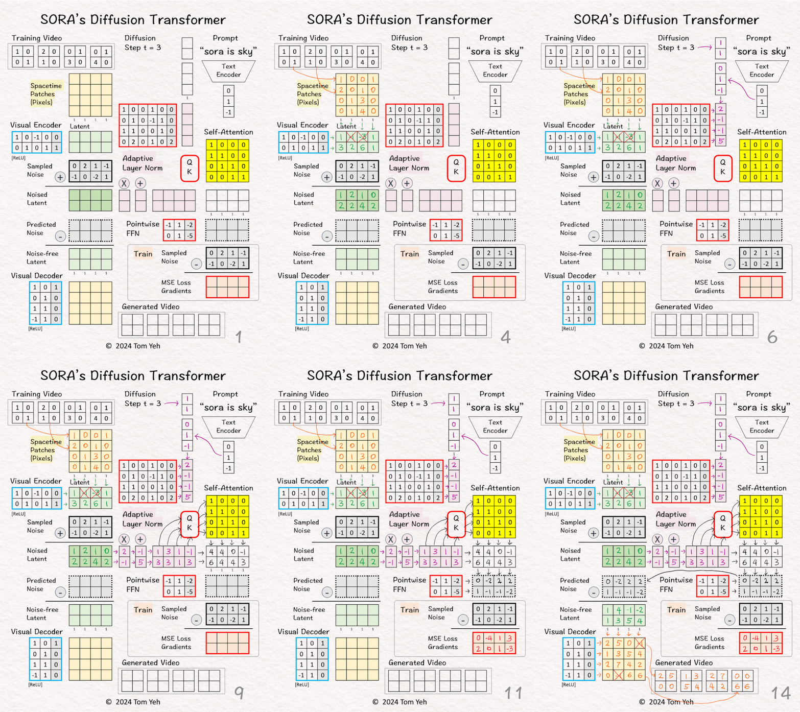
Can you calculate Sora’s Diffusion Transformer (DiT) by hand? ✍️
[Like] if you can follow the calculation.

OpenAI‘s Sora is based on the Diffusion Transformer (DiT) developed by William Peebles and Saining Xie in 2023.

How does DiT work?

— 𝗚𝗼𝗮𝗹 —

Generate a video conditioned by a text prompt and a series of diffusion steps

— 𝗪𝗮𝗹𝗸𝘁𝗵𝗿𝗼𝘂𝗴𝗵 —

[1] Given
↳ Video
↳ Prompt: “sora is sky”
↳ Diffusion step: t = 3

[2] Video → Patches
↳ Divide all pixels in all frames into 4 spacetime patches

[3] Visual Encoder: Pixels 🟨  → Latent 🟩
↳ Multiply the patches with weights and biases, followed by ReLU
↳ The result is a latent feature vector per patch
↳ The purpose is dimension reduction from 4 (2x2x1) to 2 (2×1).
↳ In the paper, the reduction is 196,608 (256x256x3)→ 4096 (32x32x4)

[4] ⬛ Add Noise
↳ Sample a noise according to the diffusion time step t. Typically, the larger the t, the smaller the noise.
↳ Add the Sampled Noise to latent features to obtain Noised Latent.
↳ The goal is to purposely add noise to a video and ask the model to guess what that noise is.
↳ This is analogous to training a language model by purposely deleting a word in a sentence and ask the model to guess what the deleted word was.

[5-7] 🟪 Conditioning by Adaptive Layer Norm

[5] Encode Conditions
↳ Encode “sora is sky” into a text embedding vector [0,1,-1].
↳ Encode t = 3 to as a binary vector [1,1].
↳ Concatenate the two vectors in to a 5D column vector.

[6] Estimate Scale/Shift
↳ Multiply the combined vector with weights and biases
↳ The goal is to estimate the scale [2,-1] and shift [-1,5].
↳ Copy the result to (X) and (+)

[7] Apply Scale/Sift
↳ Scale the noised latent by [2,-1]
↳ Shifted the scaled noised latent by [-1, 5]
↳ The result is “conditioned” noise latent.

[8-10] Transformer

[8] Self-Attention
↳ Feed the conditioned noised latent to Query-Key function to obtain a self-attention matrix
↳ Value is omitted for simplicity

[9] Attention Pooling
↳ Multiply the conditioned noised latent with the self-attention matrix
↳ The result are attention weighted features

[10] Pointwise Feed Forward Network
↳ Multiply the attention weighted features with weights and biases
↳ The result is the Predicted Noise

🏋️‍♂️ Train

[11]
↳ Calculate MSE loss gradients by taking the different between the Predicted Noise and the Sampled Noise (ground truth).
↳ Use the loss gradients to kick off backpropagation to update all learnable parameters (red borders)
↳ Note the visual encoder and decoder’s parameters are frozen (blue borders)

🎨 Generate (Sample)

[12] Denoise
↳ Subtract the predicted noise from the noised latent to obtain the noise-free latent

[13] Visual Decoder: Latent 🟩 → Pixels 🟨
↳ Multiply the patches with weights and biases, followed by ReLU

[14] Patches → Video
↳ Rearrange patches into a sequence of video frames.

POST: https://www.linkedin.com/posts/tom-yeh_gemini-transformer-deeplearning-activity-7167154366821380096-e2YQ

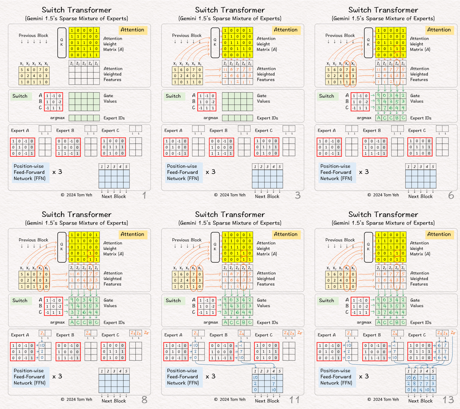
Can you calculate Gemini 1.5’s Switch Transformer by hand? ✍️
[Like] if you can follow the calculation.

Google recently released Gemini 1.5, which adds Sparse Mixture of Experts to Gemini 1.0’s architecture.

The idea of Sparse Mixture of Experts first appeared in the Switch Transformer model described in a 2022 article in the Journal of Machine Learning Research:

“Switch Transformers: Scaling to Trillion Parameter Models with Simple and Efficient Sparsity” by William (Liam) Fedus, Barret Zoph, Noam Shazeer.

How does a Switch Transformer work?

— 𝗪𝗮𝗹𝗸𝘁𝗵𝗿𝗼𝘂𝗴𝗵 —

[1] Given
↳ Input features (X1-X5) from the previous block

🟨 ​🇦​​🇹​​🇹​​🇪​​🇳​​🇹​​🇮​​🇴​​🇳​

[2] Attention Matrix
↳ Feed all 5 features to a query-key attention module (QK) to obtain an attention weight matrix (A).

[3] Pooling
↳ Multiply the input features with the attention weight matrix to obtain attention weighted features (Z1-Z5).
↳ The effect is to combine features across positions (horizontally)

[4] Visualize Pooling
↳ Z4 := X4 + X5 because the 4th column in the attention weight matrix A is [0,0,0,1,1]

🟩 🇸​​🇼​​🇮​​🇹​​🇨​​🇭

[5] Gate Values
↳ Multiply attention weighted features (Zs) with switch matrix
↳ For each weighted feature Zi, each gate value indicates how well an expert (A,B,C) can probably handle the feature

[6] Top Expert
↳ Find the row (Expert ID) with the highest gate value
↳ “Sparse” refers to the selection of only the top expert, not all the experts.

🟦 ​🇫​​🇫​​🇳​

[7] Routing
↳ Each Z is routed to the best expert
↳ Each expert has a fixed capacity of 2.
↳ Note that Z5, which is supposed to go to Expert C, exceed’s the capacity.

[8] Expert A: Linear Layer
↳ Apply the linear layer (multiply Z1 with weights and biases)
↳ The effect is to combine features across feature dimensions (vertically).

[9] Expert A: Aggregate
↳ Send the resulting combined feature to corresponding output column.
↳ The paper has an extra scaling step, omitted here for simplicity.

[10-11] Expert B
↳ Repeat [8] and [9]

[12-13] Expert C
↳ Repeat [8] and [9]
↳ However, since Z5 exceeded Expert C’s capacity, it was simply passed through as is to the next block.

POST: https://www.linkedin.com/feed/update/urn:li:share:7170458220317040640/

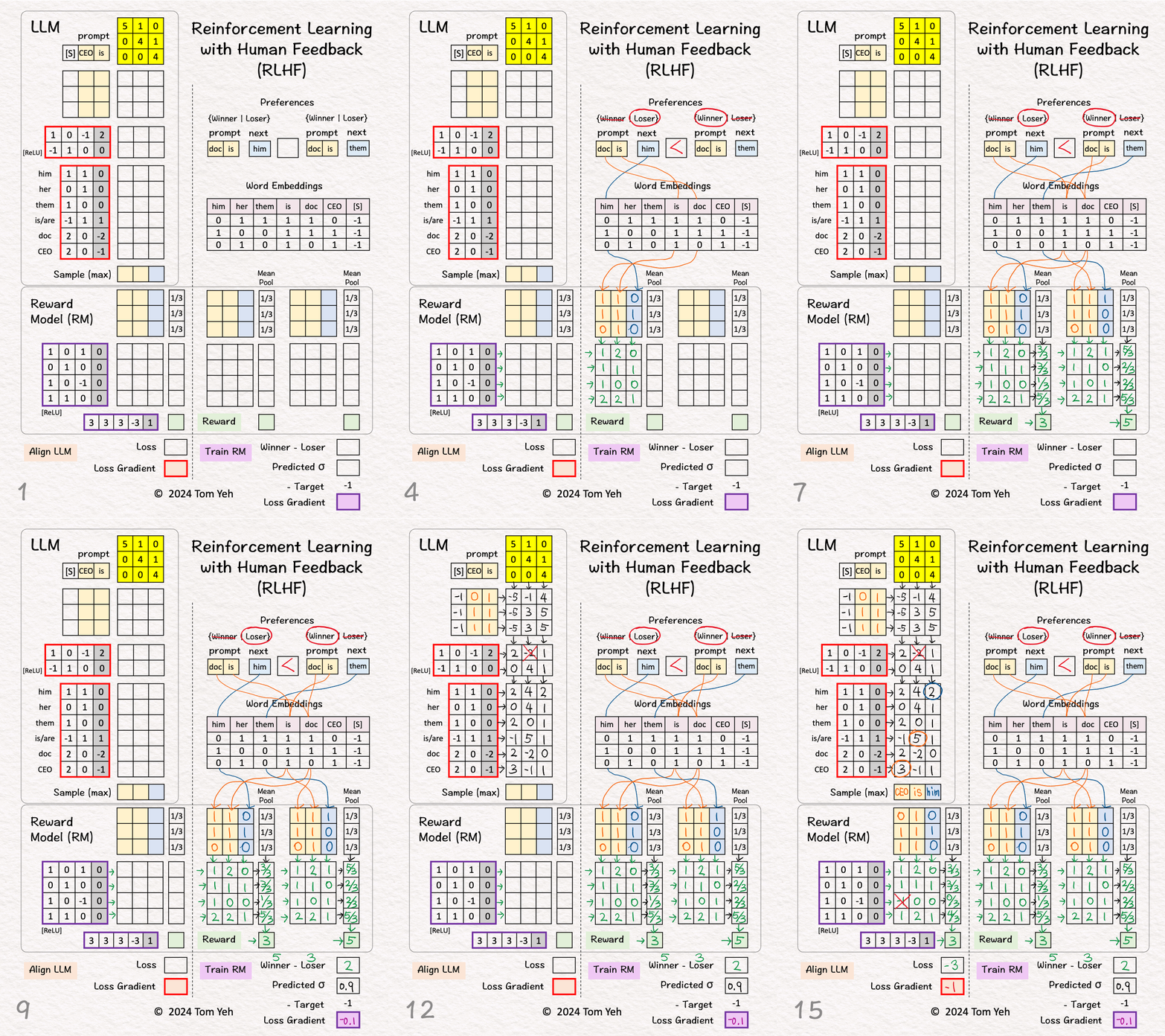
 Can you calculate RLHF to mitigate gender bias by hand? ✍️
[Like] if you can follow the calculation.

Reinforcement Learning from Human Feedback (RLHF) is a popular technique to ensure that an LLM aligns with ethical standards and reflects the nuances of human judgment and values.

Without RLHF, an LLM relies only on data and would think doctors must be men, because the data likely reflects existing biases in our society.

With RLHF, an LLM is given human feedback that doctors can be both man and women. The LLM can update its weights until it begins to use “them” rather than “him” to refer to a doctor.

Moreover, we hope the LLM not only addresses the specific bias about doctors but also learns the underlying value of “gender neutrality” and applies it to other professions, for example, learns to use “them” to refer to a CEO, even though it wasn’t explicitly taught by a human.

Claude 3 released by Anthropic, sets a new high bar for safety standards. It uses an advanced technique called “Constitutional AI” by extending RLHF, enhancing the H in RLHF with AI.

How does RLHF work?

— 𝗪𝗮𝗹𝗸𝘁𝗵𝗿𝗼𝘂𝗴𝗵 —

[1] Given
↳ Reward Model (RM)
↳ Large Language Model (LLM)
↳ Two (Prompt, Next) Pairs

🟪 TRAIN RM

Goal: Learn to give higher rewards to winners

[2] Preferences
↳ A human reviews the two pairs and picks a “winner”
↳ (doc is, him) < (doc is, them) because the former has gender bias.

[3]-[6] Calculate the Reward for Pair 1 (Loser)

[3] Word Embeddings
↳ Lookup word embeddings as inputs to the RM

[4] Linear Layer
↳ Multiply the input vectors with RM’s weights and biases (4×4 matrix)
↳ Output: feature vectors

[5] Mean Pool
↳ Multiply the features with the column vector [1/3,1/3,1/3] that achieves the effect of averaging the features across the three positions
↳ Output: sentence embedding vector

[6] Output Layer
↳ Multiply the sentence embedding with the weights and biases (1×5 matrix)
↳ Output: Reward = 3

[7] Reward for Pair 2 (Winner)
↳ Repeat [3]-[6]
↳ Output: Reward = 5

[8] Winner vs Loser’s Reward
↳ Calculate the difference between the winner and the loser’s reward
↳ RM wants this gap to be positive and as large as possible
↳ 5 – 3 = 2

[9] Loss Gradient
↳ Map reward gap to a probability value as prediction: σ(2) ≈ 0.9
↳ Calculate loss gradient by Prediction – Target: 0.9 – 1 = -0.1
↳ The Target is 1 because we want to maximize the reward gap.
↳ Run backpropagation and gradient descent to update RM’s weights and biases (purple border)

🟧 ALIGN LLM

Goal: Update weights to maximize rewards

[10]-[15] See details in the comment